The cubic splines interpolation algorithm does not work well for interpolation when the x values are large and have a large distance between them.
Under these circumstances, cubic splines interpolation becomes very unstable making interpolations incorrect by many orders of magnitude.
They are also very poor for extrapolating under these conditions.
Therefore we use an alternate polynomial interpolation method.
The Cubic splines algorithm draws a cubic polynomial between each point pair but constrains the spline to have the same derivative as the next spline at the measured points.
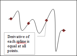
Figure 1. Cubic splines algorithm draws a cubic between each of the measured points.
There are two types of cubic splines, free and clamped.
Free splines have a boundary condition in which the second derivative at the outside end points is zero. This means there is a local maximum or minimum in the first derivative at that point.
Clamped splines enable the user to set the first derivative at the outside end points.
We will use an example from Burden et al1 Section 3.6 to illustrate. These authors attempted to interpolate between points measured on a picture of the cartoon character Snoopy.

Figure 2. Snoopy to be interpolated.
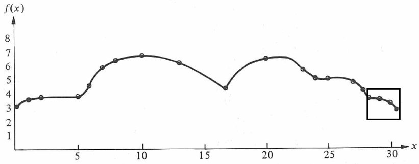
Figure 3. We used the last four points for the interpolation test.
To save time, we used only the four last points of the example. Using the data in Table 1, we were able to reproduce a fairly close approximation using Cubic Splines algorithms.
Table 1. The actual values we used from the Snoopy example.
| i |
xi |
ai |
| 0 |
27.7 |
4.1 |
| 1 |
28 |
4.3 |
| 2 |
29 |
4.1 |
| 3 |
30 |
3 |
Figure 4. Free cubic splines was a good interpolation function.
Figure 5. Clamped cubic splines was also a good interpolation function.
Extrapolation using Cubic Splines
Warning: Don’t use cubic splines to extrapolate beyond the data set! The boundary conditions for both types of splines virtually guarantee that the spline will not follow the trend of the points. Even if you use a clamped spline with the boundary condition that the first derivative is zero at the outside end points, these become a local minimum for the interpolation function.
In our Snoopy example both were poor functions for extrapolation.
The free cubic spline specifies the second derivative = 0 at the end points. This produces a local minimum or maximum in the slope of the interpolation. This is not useful for extrapolation purposes.
Figure 6. Free cubic splines shows odd linear extrapolation behavior.
In the clamped cubic spline we set the boundary conditions so that the first derivative at the end points is zero. This makes the endpoints a local minimum or maximum. This strategy is sure to destroy any attempt at extrapolation.
Figure 7. Clamped cubic splines extrapolation is very poor.
Cubic Splines sensitive to horizontal scale
In addition to extrapolation problems, the cubic splines algorithm is very sensitive to scale of the independent variable. We multiplied x values by 1000 in the Snoopy example and found surprising results.
The cubic splines algorithm produces surprising oscillation and instability when the independent variable scale is large and data measurements are sparse.
Figure 8. Free cubic splines produces surprising oscillation.
These algorithms are not for interpolation across large distances.
Figure 9. Clamped cubic splines shows the same instability but worse extrapolation utility.
Warning: Don’t use cubic splines to extrapolate beyond the data set! The boundary conditions for both types of splines virtually guarantee that the spline will not follow the trend of the points. Even if you use a clamped spline with the boundary condition that the first derivative is zero at the outside end points, these become a local minimum for the interpolation function.
Why is this all a problem for reservoir engineers?
Our problem is interpolating measured reservoir pressures in a pool. Pool pressure measurements are usually taken once per year or even less frequently. Some pools have no pressure records for an entire decade. Yet we must have an adequate way to interpolate and even extrapolate these pressures over the life of the pool.
Production is measured monthly. At minimum, we will need a dozen interpolation points between each measured pressure points.
In the problem of interpolating measured reservoir pressures for a pool, the independent axis is a time scale which can be very large scale. Pools produce for decades which is on the order of 103 days on a scale that might start near 20,000. For this type of measurement period, cubic splines is highly unstable and oscillatory.
Extrapolation using cubic splines doesn’t produce believable pressures.
Clearly a better interpolation system is required for this type of system.
Alternate solution
As a solution, this algorithm draws a cubic through four points.
It calculates the parameters of the polynomial
y = a x3 + b x2 + c x + d
This forces the cubic to be a close interpolation to the curve of the measured points. It also allow for realistic extrapolations. Size of horizontal scale does not impact the interpolation results.
The proposed method is designed to be used for the interpolation between the middle points and to provide a reasonable extrapolation.
The downside of this alternative is that this function is not analytically differentiable.
The algorithm uses each set of internal four points to calculate a well behaved cubic spline to be used in the middle points.
- Where there are no points on one side, use a constant value
- Where there is only one point on both sides, use a constant slope
- Where there is only one point on one side, use a parabolic fitted through three points.
- Where there are two points on either side, use a cubic fitted through four points.
Figure 10. Snoopy interpolated by proposed algorithm.
Figure 11. Proposed algorithm interpolates smoothly and extrapolates well.
1Burden, Richard L., Faires, J. Douglas, and Reynolds, Albert C., Numerical Analysis Second Edition, Wadsworth, Inc., 1981.